It’s the summer of 2026 and betting is very cool. You just do not want to be caught watching a World Cup game without having done a 17-leg parlay. You get to say things like “this match is so mispriced” or “I’m going to buy insurance on my country losing”. For max street cred, during hydration break, drop a “my analyst at D.E. Claw just pinged me on Telegram, they’ve found a sick +EV trade”.
However, people trading stuff in seemingly complex ways and bizarre jargon is not a new phenomenon as volatility traders have been around for a long time. In fact, institutionally dealing with contracts that depend on the outcome of more than one event, such as Kalshi’s combos and Polymarket’s parlays, is among the main sources of income for French people in NYC and London.
It turns out, pricing these bets is all about correlation. And correlation trading is something vol traders think a lot about, particularly for one kind of strategy called dispersion.
Pricing a parlay
A parlay is simply a bet on two or more events - it pays off if all its legs hit, so its price must depend on the joint probability distribution of its legs.
Take the simplest parlay: two legs, A and B, each a coin flip. We can visualize the whole outcome space in a 2x2 grid, seen below. Green denotes the probability that the parlay hits as both events land, so its price should mostly be determined by this area. Change the correlation between these events by dragging the slider or choosing a number directly to see how it impacts the price.
As is to be expected, higher correlation makes the green area larger and therefore increases the price of the parlay (there is no free lunch, since you also have a higher probability of winning). But also notice how the vertical divider never moves: correlation is about how the diagonals compare to each other, while the columns are about marginal probabilities. Said otherwise, individual leg prices contain no information about parlay price beyond the independence baseline.1
What does this mean for your sports betting? Well, a bet on “Lakers win vs Warriors AND Celtics win vs Knicks” has a fair correlation of basically zero, as the games happen in indoor stadiums, at different times, in different parts of the country. A bet on “France wins vs Argentina AND Mbappé scores” should not have a fair correlation of zero, as the probability of France winning is not the same given an Mbappé goal as opposed to no goal. Of course, whoever is selling you the parlay knows this and they will offer you that correlation at a premium to fair to make some money.2 In fact, to spot this in the wild, go ahead and price a two-leg parlay on some NBA games and back out the implied probability off of the individual leg prices. You just paid for a market maker’s lunch!
What does this have to do with options?
Now, instead of two coin flips, consider an option on a basket of two stocks, each with 50% weight. Though it may sound like an intimidating jump, they are fundamentally similar in that both a coin flip and a stock’s return are random events, with their respective potential outcomes and attached likelihoods. The key difference is that we move from a discrete world (of binary events such as “heads or tails” or “Knicks win or lose”) to a continuous one (a stock’s return is described by a probability distribution). The neat thing is that the main learnings from the previous section still stand and, notably, the largest difference is that instead of looking at a 2x2 grid we now look at a “cloud” of dots, all of which represent a draw from the joint probability distribution of the two stocks.
So, for higher correlations, more dots end up “in-the-money” (i.e. in the green-shaded area) which means a more expensive option. And still, the marginal distributions remain the same after changing the correlation.
This is directly related to why “worst-of options” are so popular in structured products world. These contracts work just like vanilla options except that at maturity they pay the return of the worst-performing stock in a given basket. Since an option price is just the present value of some weighted-average of payoffs at maturity, worst-of pricing is particularly sensitive to correlation:
- Higher correlation between component stocks pushes more dots into the in-the-money area (shaded green below), therefore a holder of the option expects to make money in more future paths of the world
- Higher correlation pulls the minimum return towards the average, therefore not only do you as holder of option make money in more paths, you make more money on those paths!
What does this mean if you are a structurer at a bank? Well, clients generally like more exposure to stocks per unit of premium, so a cheaper option makes a product more attractive. So you should be excited to offer more upside to your client! Which depends, of course, on your sales contact’s generosity towards splitting client upside with their own mark-ups: after all, a cheaper product means you can sell the same quantity for higher margin.
The market price for correlation
Listed equity options are typically single stock (the underlyer is NVDA) or index (the underlyer is the S&P 500) contracts. The S&P 500 index, in and of itself, is a basket not unlike the one described in the toy example above, implying that an option on the index is effectively a basket option, which must mean the market prices some level of correlation for its constituents. How could we go about finding this price out?
We have implied volatilities from both single stock and index options quoted on the market. A quick trip down memory lane gives us that if stock \(i\) has weight \(w_i\), the index variance is:
$$\sigma_I^2 = \sum_{i=1}^{N} w_i^2\,\sigma_i^2 + 2\sum_{i \lt j} w_i w_j\,\rho_{ij}\,\sigma_i\sigma_j$$where \(\rho_{ij}\) is the correlation between stocks \(i\) and \(j\). Everything in this equation is readily available, except for the correlations and, since we have \(N(N-1)/2\) of them but only one equation, we’ll need to take a shortcut and assume that every pair shares correlation \(\rho\). Solving for it gives:
$$\rho = \frac{\sigma_I^2 - \sum_i w_i^2\,\sigma_i^2}{2\sum_{i \lt j} w_i w_j\,\sigma_i\sigma_j} $$This is what people generally call implied correlation. Expanding the index variance term and after a quick bit of algebra:
$$\rho = \frac{\sum_{i \lt j} w_i w_j\,\sigma_i\sigma_j\,\rho_{ij}}{\sum_{i \lt j} w_i w_j\,\sigma_i\sigma_j}$$This shows that correlation is actually a normalized weighted-average of pairwise correlations, where the weights are proportional to risk as given by the product of the stock’s weight in the index and its volatility.3
Note, however, that by taking as inputs option market prices, we would’ve had to choose some strikes (traditionally, 50-delta) and some tenor (typically, 3 months) - which, in turn, means that implied correlation has its own surface akin to that of volatility. Yes, this means that implied correlation has its own term structure and skew!
Finally, by trying to answer “what correlation does the market price in for S&P 500 constituents”, we have approached things from an implied perspective. Trading options is about implied versus realized. However, the above is agnostic to implied versus realized and switching worlds simply changes where the volatilities come from: market prices versus historical estimates.
How to trade correlation?
The variance equation outlined previously gives us a hint: if index variance is comprised of single stock variances and some correlation component, correlation is likely traded by playing index variance versus its single stock counterparts. That’s what dispersion trading is all about.
Still, dispersion can be structured in many ways. In addition to the usual choices of strike and tenor, you can source volatility (or variance) exposure from many different instruments: delta-hedged options, strangles/straddles, or variance/volatility swaps. In practice, most people won’t choose to trade a perfect basket of stocks (e.g. all components in the S&P 500), but instead choose a sensible subset such as the top 50 or 100 largest names. Further, dispersion generalizes to the relative value trade of the volatility of any basket versus the basket of its components’ volatilities (for example, tech/AI/semiconductor dispersion was very topical in early 2026).
Each construction decision has its own trade-offs. For the following bit, we’ll assume variance swaps as their constant gamma profile makes the explanation simpler.
Let’s assume \(\rho_{ij} = \rho\) and define index variance as the combination of diagonal terms, related to individual stock variance, and off-diagonal covariance terms:
$$\sigma_I^2 = \sum_{i=1}^{N} w_i^2\,\sigma_i^2 + 2\sum_{i \lt j} w_i w_j\,\rho_{ij}\,\sigma_i\sigma_j = D + \rho C$$A pure correlation trade should have no opinion on how much variance is realized, therefore a good starting point is to buy and sell equal amounts of variance on each of the legs. Index variance embeds variance across the whole covariance matrix while stock variance is only about the diagonal, so trading the former against the latter by construction will result in net exposure to the covariance terms. If we sell some index variance and buy the same amount of total stock variance (weighted properly), it must be the case that we are short the off-diagonals and long the diagonals and that’s precisely how we isolate our P&L to correlation:
The anatomy of index variance
An index contains each stock's own variance on the diagonal and every pair's covariance off it. Correlation fills only the off-diagonal cells.
For the slightly more algebra-inclined: say we short one unit of index variance and buy \(\lambda w_i^2\) of each name’s variance. At expiry, the short leg pays \(\sigma^2_{I,impl} - \sigma^2_{I,rlzd}\) and the long leg pays \( -\lambda(D_{impl} - D_{rlzd}) \). Plug in \( \sigma_I^2 = D + \rho C\) on both sides:
$$\Pi = (D_i + \rho_i C_i) - (D_r + \rho_r C_r) + \lambda (D_r - D_i)$$Regroup the single stock variance (\(D\)) terms and you get:
$$\Pi = (\lambda-1) (D_r - D_i) + \rho_i C_i - \rho_r C_r$$Now, one could very reasonably assume \(\lambda = 1\) is a good solution. Yet, we can rule that out from first principles: if we short one unit of index variance and long single-name variance in weights \(w_i^2\), we are simply neutralizing the diagonal terms. Individual stock variance carries no off-diagonal content, so we must be exposed to covariance, which, in turn, is related to volatilities and correlations. Therefore, our bet is still not a pure correlation one.
No wonder vol trading is such a great nerd-sniping weapon! All we wanted was to trade some correlation…
Ideally, the trade P&L should be zero whenever realized correlation matches implied, regardless of what the vols did. So let’s assume \( \rho_r = \rho_i = \rho \) and also that vols realize at a multiple \(c\) of implied:
$$\Pi = (c^2-1) [(\lambda-1) D - \rho C]$$Solve the bracket for the fair game of zero P&L:
$$\lambda = 1 + \frac{\rho C}{D} = \frac{\sigma_I^2}{D}$$The excess over the naive weight is a long position in single-stock variance, sized to exactly the \( \rho C\) of covariance we were originally short. Finally, the P&L boils down to:
$$\Pi = c^2 C (\rho_i - \rho_r)$$While \(c^2 C\) scales the economic result, the sign of P&L is solely determined by the spread between implied and realized correlations, as we originally intended. Since we sold index vol and purchased stock vol, we benefit from a high implied level and a low realized one, which is usually referred to as being short correlation. That’s the core exposure of the dispersion trade.
This weighting scheme is theta-neutral: theta is the rent paid for realized variance exposure (dollar-gamma, to be precise). If volatilities all move the same way in relative terms (i.e. all vols increase by 10%, so index goes up from 20 –> 22 and stocks from 30 –> 33), the strategy should remain flat. However, the strategy is short vega and will lose money if vols instead move the same in absolute terms (i.e. all vols increase by 5v, so index goes up from 20 –> 25 and stocks from 30 –> 35). This is because single stock vol is higher than that of index: stock vol is richer in variance per unit than index and, therefore, we need to hold less of it. Or think about it another way: consider implied correlation an exchange rate between index and stock variance. Theta-neutral dispersion attempts to size its legs equally at that exchange rate. So, the ratio of single-name to index variance on a theta-neutral dispersion portfolio must be related to the implied correlation!4
As a result, a vega-neutral weighting requires, for the same index leg, buying more single stock vol than theta-neutral. It is, then, generally seen as a more balanced construction alternative to theta-neutral due to being a correlation trade (theta-neutral) plus a long single-stock vol overlay. Vega-neutral dispersion breaks even if all vols move the same in absolute terms (same increase in vol points). While a trader sizing in theta-neutral fashion cares more about the ratio of single stock to index vol (or its square, to be precise), a vega-neutral trader will pay more attention to the difference (spread) between those vols.
When and why does dispersion make money?
Being short correlation means you make money if the average correlation between index constituents is low (or, more precisely, when realized correlation is below the level sold at). That’s where the strategy gets its name from: higher cross-sectional dispersion among stocks means, all else equal, that their realized correlation will be lower. Picture a day where GOOG is up a ton while AMD tanks or all tech/semi stocks are going to the moon while the rest of the index is flat: all of those are symptomatic of low realized correlation and great for dispersion strategies.
But that’s only one piece of the puzzle. Broadly speaking, a dispersion book deals with two main sources of uncertainty:
[1] Single-stock vol premium: did the names move more or less than their options implied?
[2] Correlation premium: did the names move together more or less than was implied?
Hopefully, the previous section illustrated that the question of how to size the two legs of the trade essentially boils down to what kind of exposure profile one wants in terms of the two premia above. Theta-neutral dispersion, as a pure correlation trade, attempts to isolate [2] and get rid of [1]. More defensive constructions, such as vega- and gamma-neutral5, introduce more of [1] in the mix.
But why should anyone expect to make money on this?
It would make me feel a lot cooler to claim that any of the above is alpha, but it’s really just fancy beta: you should expect to earn positive expected return over time by trading dispersion because you are taking on risks that other players in the market want to offload. Exactly the same reason one expects to make money holding stocks or selling hedged options over the long-run: risk premia.
That’s not to say there’s no alpha in dispersion! There are many ways to generate it: stock picking (choosing custom baskets of stocks which screen particularly attractive), timing (knowing when to enter/exit or sizing of exposures through time), and even option picking (targeting specific corners of the vol surface). And, as for all vol strategies, you can try to add some value by hedging in a specific way, such as using different models for delta calculation or even by making outright calls about hedge sizing.
And who exactly is paying for this risk premium? At a very high level, two types of flows are usually behind it: index options are one of the main ways for purchasing insurance against a crash in equities, so the relative excess demand for index volatility pushes its implied volatility up. The single-stock space, on the other hand, has a larger presence (for the size of the market) of flows arising from hedging activity of structured product issuance (remember worst-of options?) and call-overwriting programs, both of which have the effect of supplying stock volatility and therefore bringing implieds down.
As with any risk premium, its magnitude varies over time and the last few years have been remarkable ones for correlation. The chart below plots implied and realized 3-month correlation for the top 50 stocks in the S&P 500:
- Implied correlation is simply CBOE’s COR3M Index, which is available publicly and in fact calculated using the methodology described above
- Realized correlation is my vibe-coded implementation using publicly available sources and attempts to replicate CBOE’s COR3M methodology but for realized corr, using historical vols and pairwise correlations and plotted at quote date (i.e. the realized correlation for 15Jan2020 is the subsequent 3m one) so that it covers the same timeframe as implied and those two are therefore comparable
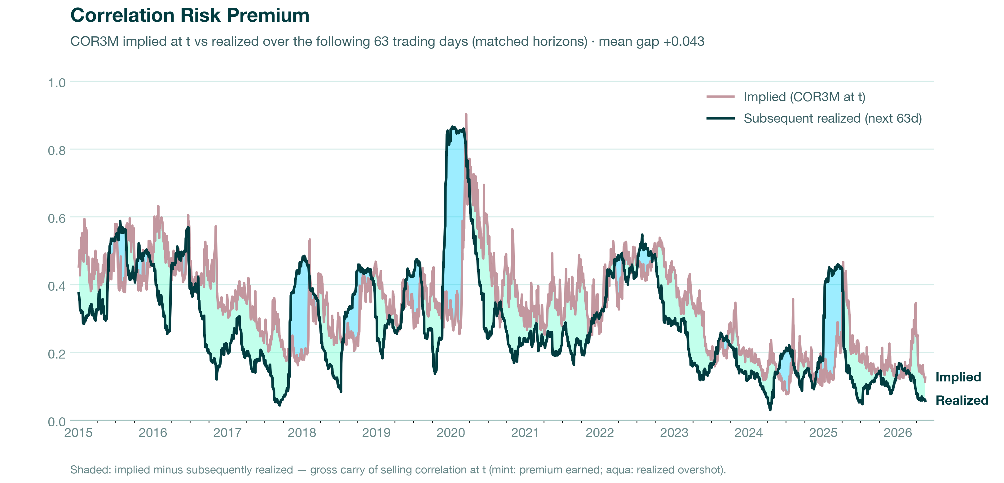
It stands out that correlation has been consistently low since 2023. It’s hard to pinpoint precisely the reason for this: guesses can range all the way from more mechanical hypotheses (massive rise of index option selling programs suppressing index vol, while larger concentration among index constituents and blockbuster earnings surprises raise stock vol) to shifting market narratives (such as, since the launch of GPT 3.5, AI-adjacent stocks gained a lot of significance in the index and have behaved very differently from the rest of stocks, thereby decreasing correlation).
Personally, the most remarkable thing about this period is how great a case study it provides in how trading vol solely based on implied levels can go wrong. Effectively, implied correlation touched its all-time low in the summer of 2024. 0th percentile! How can you not want to buy something that is stationary and at the very bottom of its historical distribution? Well, implied is not the full picture and what the last few years have taught us is that realized can always go lower.
In sum
As far as betas go, dispersion is a tricky one but, with any luck, this has shed some light on the key dynamics behind it. I would feel my job is done if I helped generate the slightest bit of suspicion the next time you read “parameter X is at such a low (high) percentile so don’t miss out on the chance to buy (sell) it”!
Unfortunately, at the time of writing this article, we cannot yet trade NBA dispersion on Kalshi. Try computing the implied correlation of a multi-leg parlay (for different games), check that it is not zero and (hopefully) after reading this, you will think “I should short it!”… but life is not so simple.
To be precise, individual leg prices do contain some information about a parlay price: they impose bounds. They simply do not uniquely determine it without a dependence assumption. ↩︎
This is why sportsbooks restrict, reprice, or outright refuse certain same-game combinations: the dealer won’t put money where their mouth is if the model is shaky. ↩︎
I like to think of the denominator as the total covariance capacity of the index constituents (the amount of co-movement they would display if they were all perfectly correlated), while the numerator denotes the actually realized co-movement of stocks. Correlation is, then, simply the share of total covariance capacity that is actually carried through. ↩︎
It’s worth explicitly pointing out that correlation lives in variance space. Vega lives in vol space, therefore the ratio of single-stock to index vega is approximately the square-root of implied correlation. ↩︎
So far, I have ignored gamma-neutral dispersion here as I think of gamma-neutral as a long stock vol trade partially financed by some correlation premium, but not quite a correlation trade. ↩︎